Who is this for

This article assumes you have a basic familiarity with the concept of asymptotic runtimes, typically talked about using big O notation. And it also assumes a familiarity with recursive functions and trees.

Motivation

Recursive functions can be hard to reason through when thinking about their runtime analysis. It's also not always clear how each additional recursive call affects the total runtime of a recursive function.

To help with this, this is a short reference article noting models to use when thinking about recursive functions, building from explanations on the topic in Cracking the Coding Interview.

The models

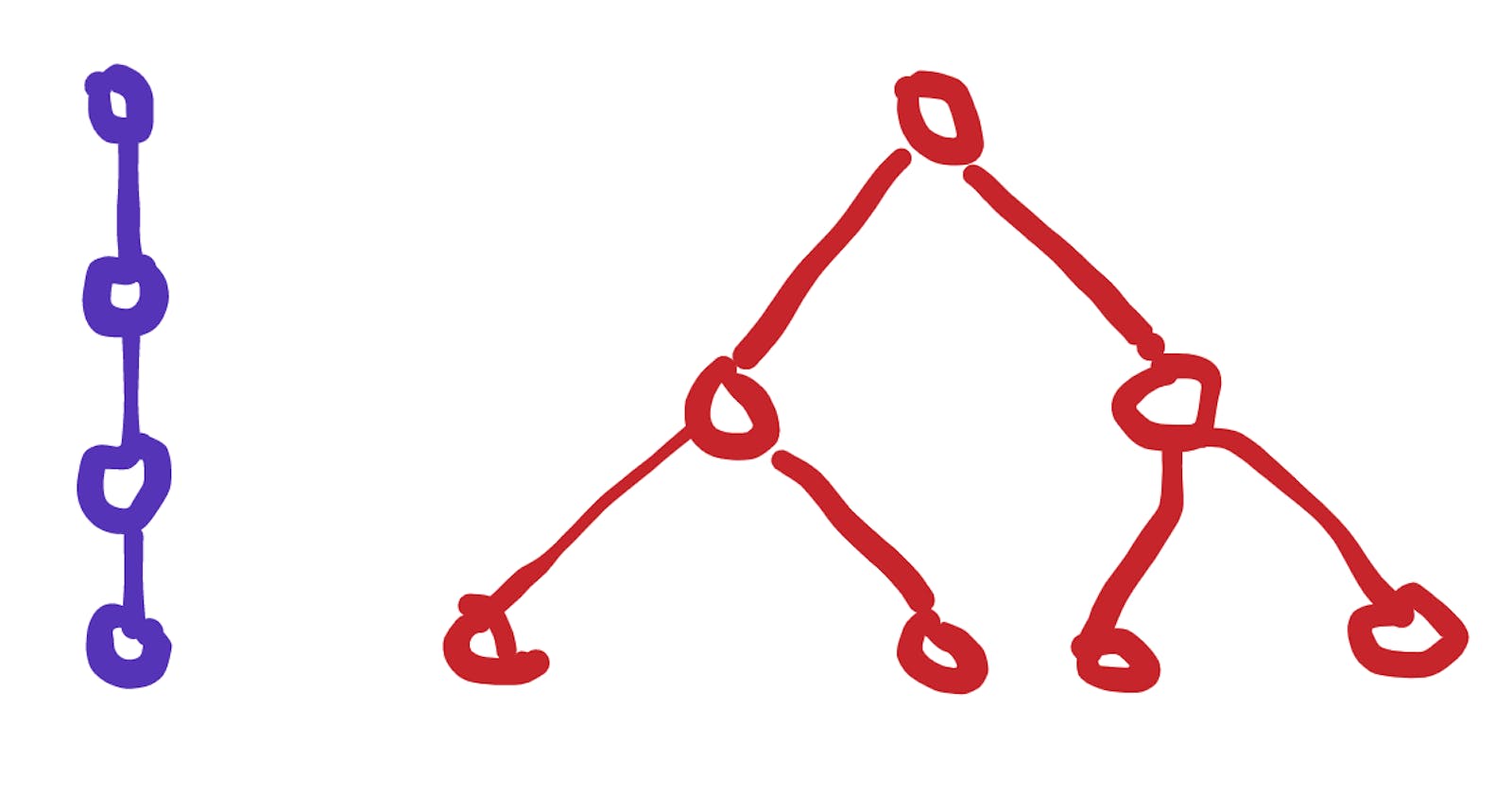
Picture a tree, sort of like a family tree:

and a list, very much like an array:

A recursive function with only direct recursive calls will create a call stack that looks like one of these two models, which can be studied as data structures in their own right. It will always start with a parent node, and branch out or down into child nodes, and each node will end up doing a fixed amount of work.

To determine the runtime of the recursive function, the basic idea is to:

1. use these models to help determine the number of nodes that will exist in the call stack.
2. determine how much work each node in the tree or list will do.
3. sum up all the work done by every node to give the total work that will be done by the recursive function.

1. Use # of direct recursions to choose model

By the number of direct recursions we mean the number of statements in the function's body where the function calls itself.

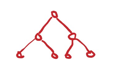
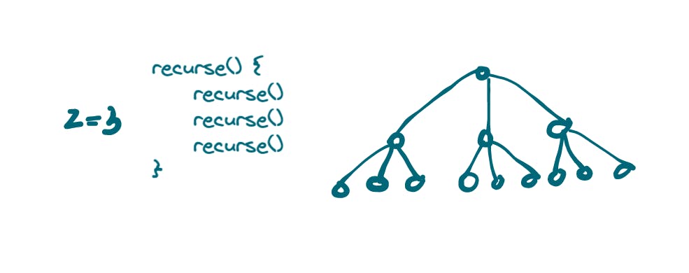
A recursive function with two direct recursions creates a tree that resembles a perfect binary tree,

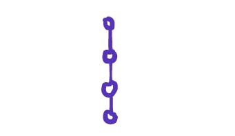
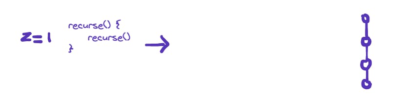
while one with just one direct recursion creates a tree that resembles a list.

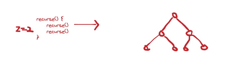
We'll call this number, the number of direct recursive calls z. And we can have recursive calls with z > 2 such as:

2. Determine number of nodes in a model

When z = 1

If z=1 then we know we can use a list to model the call stack. In which case the number of nodes in the list will be the number of times the recursive function was called. Now here's a challenge:

How many times will the function, recurse, be called starting with n = 5?

recurse(n) {
  if(n===1) return
  recurse(n-1)
}

recurse(5)

When you figure out what that number is, let's call it the depth of our tree, that will be the total number of nodes we'll have.

When z > 1

If z >1, we know we'll have a tree. But even though it's typically straightforward to figure out how many times our function will be called, again, let's call this the depth of our tree, it's not always so straightforward to figure out how many nodes exist in the tree, especially when the depth is very large.

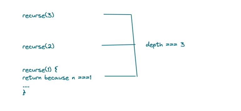
Here's another challenge. What's the depth of the tree formed when we call recurse(3).

recurse(n) {
  if(n===1) return
  recurse(n-1) // z > 1 because recurse calls itself 2 times
  recurse(n-1)
}

recurse(3)

I'll help out this time. The depth is 3. Here's a representation of one line of execution on the call stack to show how it's 3.

But this doesn't give us the full picture to help determine how many nodes will exist in total. Here's the full picture:

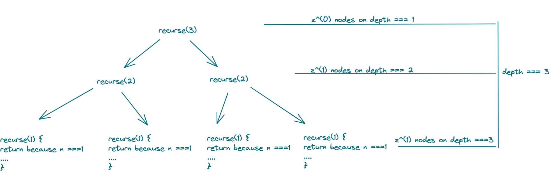
Take note of the pattern that evolves as a function of the number of direct recursions, z. In this example, the number of direct recursions in recurse is 2, z=2.

Note the pattern:

• depth 1: z^(0) nodes
• depth 2: z^(1) nodes
• depth 3: z^(2) nodes

When we substitute in z=2, this gives

2^0 + 2^1 + 2^2 = 7

nodes in total.

Thankfully, this is a common summation pattern that can be expressed as

The sum from n = 0 to n-1 of 2^n is (2^n) - 1

More generally, the sum from n=0 to n-1 of some number P^n is ((P^n) - 1)/(P - 1)

It's important to note the general case, noting that the sum becomes some constant c * P^n. This is important because it tells us that if we try to get the exact number of total nodes in a tree with z == 3 using (3^n) - 1 we'll get a wrong answer. But we're not looking for exact.

As long as asymptotic runtimes are concerned it's alright to say when z === 3, we have O(3^n) nodes in the call stack even though the actual total is lower. This is because we ignore constants and lower power terms when working with big O.

Which leaves us with the conclusion that when z > 1 and we know the depth of the tree, the total nodes in the tree can be upper bounded asymptotically by:

3. Sum up work done

Typically, we're looking at a fixed amount of work done in each node, corresponding to O(1) or O(n) or O(logn), e.t.c

In which case our big O runtime can be surmised as:

z^depth * runtime_per_node

For example, here are the corresponding upper bounds for recurse functions by z, where each node does O(1)

• z = 1 => 1^n * O(1) = O(1)
• z = 2 => 2^n * O(1) = O(2^n)
• z = 3 > 3^n * O(1) = O(3^n)

and if recurse did O(n) work per node as in

recurse(n) {
  if(n===1) return
  for each item i in n {
    n = n+1
  }
  recurse(n-1)
}

then those runtimes become:

• z = 1 => 1^n * O(n) = O(n)
• z = 2 => 2^n * O(n) = O(n2^n)
• z = 3 > 3^n * O(n) = O(n3^n)

Sometimes, like in merge sort and binary sort, each subsequent node is doing significantly smaller and smaller amounts of work, so much so that the naive upper bound derived from this approach is actually much larger that it really is, albeit correct as an upper bound. Just not very useful.

In these cases it pays to be knowledgeable of the master method.

Conclusion

Given a recursive function with z direct recursive calls, and a depth, d, where each node does O(w) work, the runtime can be upper bounded by O((z^d) * w).

However, take care when each subsequent node is doing a significantly smaller amount of work, as that upper-bound can typically be more tightly bound to a linear or super linear runtime using the master method, as is the case in merge sort and binary search where naive upper bounds of O(n^2) and O(n) respectively, can be tightly bound to O(nlogn) and O(logn) respectively.

Thought references

Naive merge sort and binary search analysis

With merge sort z = 2, because there are only 2 branches in each call, the depth = logn, because each branch gets n/2, and work done by each node is n, because we merge n items worst case in each node. In total we get 2^logn nodes x O(n) work per node = n x n = O(n^2).

With binary search z = 2, because there are only 2 branch statements in each call, the depth = logn, because each branch gets n/2, and work done by each node is O(1), because we simply do a size comparison in each node. In total we get 2^logn nodes x O(1) work per node = n x 1 = O(n).

Corrections to naive merge sort and binary search analysis

In reality, each node in merge sort does work that's a logarithm of n, giving us O(n nodes * log n work per node). While in binary search it's a mistake to think that there are always 2 recursive calls from each node. Even though there are two recursive statements, in each node only one of those statements is ever executed, leaving us with a list instead of a tree, and a runtime equal to the depth, logn.